A common approach to source separation is to estimate a masking matrix that can classify each pixel of an Short-Time Fourier Transform (STFT) of the mixture signal into the sources.

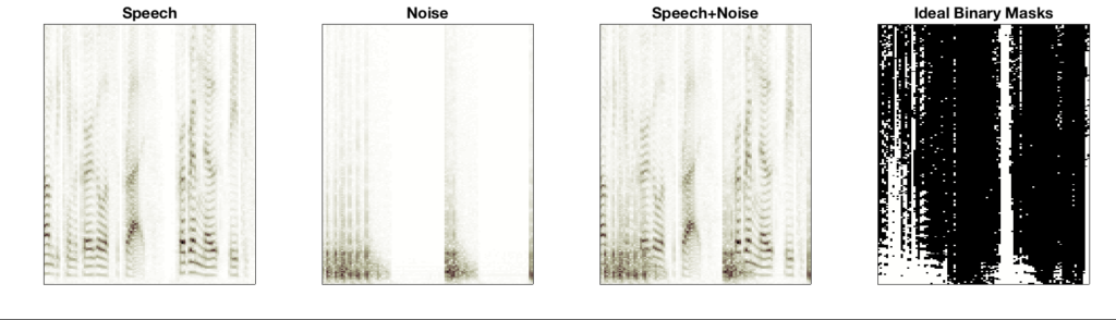
If we knew the sources, we can simply compare their pixel-wise energy and create the binary masking matrix: “1” for the pixels where speech source pixels are louder than noise and “0” for pixels with louder noise. But, what if we don’t know the sources? Well, you can try to build a supervised machine learning model, such as a deep neural network (which is another topic of research at SAIGE), but for this project we try to formulate it as a posterior estimation problem: estimating the a posteriori probability of a spectrogram pixel belonging to the source of interest given the pixel intensity of the mixture (magnitude) spectrogram. In the neural network-based approaches, the network is trained to predict the posterior probability, which is nothing but a per-pixel logistic regression problem. With Nonnegative Matrix Factorization (NMF) or Probabilistic Latent Semantic Indexing (PLSI), we directly estimate the posterior probability by using pre-trained source-specific dictionaries. More specifically, once you have a dictionary trained from clean speech and another one from noise, we can use them as the fixed basis vectors (or topics) during separation. Therefore, the test time separation process boils down to estimating the activation of those basis vectors. Finally, if we collect all the basis vectors and their temporal activation of a specific source, they reconstruct the contribution of that source to the mixture, which corresponds to the posterior distribution we want.

They all sounds good, but the procedure involves an EM-like iterative algorithm. Furthermore, obviously all the operations are on floating-point numbers. When it comes to a real-time speech enhancement system running in a small embedded system, this could be a burdensome task, because most of the time those small devices are not with enough resources (e.g. power and memory). To resolve this issue, we redefined this posterior estimation problem by using bitwise operations and binary variables.

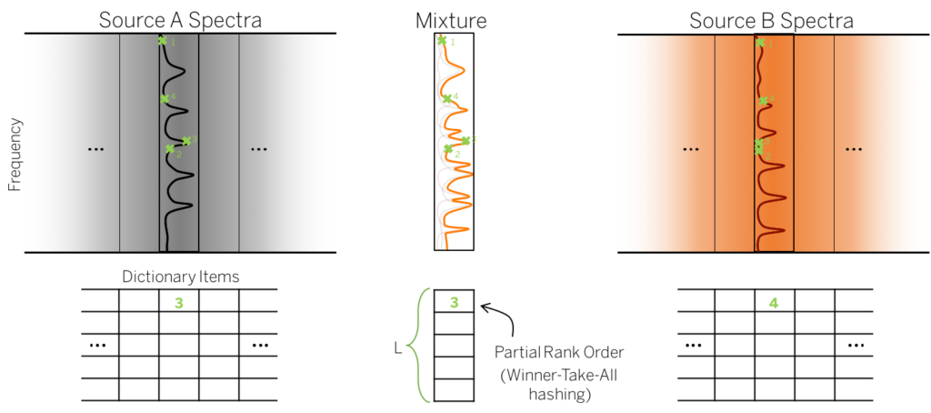
To this end, we use the concept called “partial rank order metric.” For a given mixture spectrum, we believe that there must be a pair of dictionary items, one per source dictionary1), which mix up the observed spectrum. How are we going to find out them? Maybe we can’t, but we believe that a “part” of this multidimensional vector (the mixture spectrum) must be more similar to the same part of one source than the other one. For example, if there was a high peak in Source A, while Source B doesn’t have one at the same frequency, in the mixture spectrum the peak should be preserved and an algorithm should be able to tell that the peak is from Source A. Based on this assumption, we use random sampling to find out those dominant peaks in the spectra. Let’s say that we select four random frequencies from all Source A, Source B, and mixture spectra. They are random, but the random indices should be fixed for this round. In the above figure, you see that the third frequency in Source A spectrum (the ground truth source spectrum) has a high peak. This will be the winner of the four random dimensions. We record the index of the winner in the table. But, for Source B spectrum, we don’t see a peak at the third sample, and that’s why the fourth sample is the winner of the four instead. Finally, as the third sample in Source A is so high, it’s preserved in the mixture, giving us the same winner index (number three) for the mixture random samples. We repeat this random sampling for L different times to construct an integer vector per spectrum, which look like the picture below.

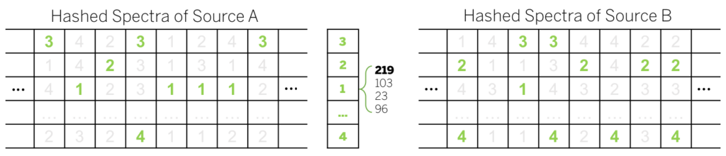
Once we convert the dictionaries and the mixture spectrum into hashed spectra this way, we can calculate the posterior probability in a bitwise fashion. For a given integer value of the mixture (“1” in the figure), we find out how many “1”s are there in the hashed Source A spectra. Suppose there are four of them. On the other hand, there is only one “1” in Source B hash codes. From here, we can assume that the winner of the four (219th frequency in the original spectrum) is more common in Source A than in B. Therefore, we can calculate the posterior probability for the 219th frequency based on the counts of matches as follows:

   

where  is the masking variable for the 219th frequency at t-th frame (0 for Source B and 1 for Source A), while  is the corresponding (219,t)-th pixel in the mixture spectrogram.  stands for the number of matches that corresponds to the 219th frequency.

This approach is advantageous because now the dictionary is a set of hash codes, which will save a lot of memory space. The operation for matching can be done in a bitwise fashion (bitwise AND), followed by pop counting. We know this algorithm sounds crazy, because it has no iteration, no real-valued parameters. You may wonder if it works. Let’s check out the results.

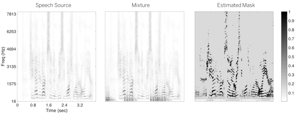
The figure is the separation result. The speech source is contaminated by a machine gun noise which is a low frequency impulsive sound. Note that the estimated mask can find out the noise component as the masking values near zero (white pixels). It of course doesn’t sound as good as the result from proper real-valued models, but the separation results are surprisingly good considering its compact structure. Let’s listen to them:

Check out our paper¹ about this.

1. Lijiang Guo and Minje Kim (2018), “Bitwise Source Separation on Hashed Spectra: An Efficient Posterior Estimation Scheme Using Partial Rank Order Metrics,” in Proceedings of the IEEE International Conference on Acoustics, Speech, and Signal Processing (ICASSP), Calgary, Canada, Apr. 15-20, 2018. [pdf][↩]