Speech/audio coding has traditionally involved substantial domain-specific knowledge such as speech generation models. If you haven’t heard of this concept, don’t worry, because you might be using this technology in your everyday life, e.g., when you are on the phone, listening to the music using your mobile device, watching television, etc. The goal of audio coding is to compress the input signal into a bitstream, whose bitrate is, of course, smaller than the input, and then to be able to recover the original signal out of the code. The reconstructed signal should be as perceptually similar as possible to the original one. 

We’ve long wondered if there’s a data-driven alternative to the traditional coders. Don’t get me wrong though—our goal is to improve the coding efficiency with the help from deep learning, while we may need to keep some of the helpful techniques from the traditional DSP technology. We are just curious as to how far can we go with a deep learning-based approach.

Our initial thought was simple: a bottleneck-looking autoencoder will do the job, as it will reduce the dimensionality in the code layer. The thing is, the dimension reduction doesn’t guarantee a good amount of compression, if each dimension should be represented with too many bits. The code has to be binary. A counterexample would be the case where the number of hidden units (or features) in the code layer is larger than the input, while the coding gain could be still high since each feature is encoded by only one bit. In other words, the encoder part of the autoencoder has to generate binarized features, not the regular real-valued ones. The binary features complicate backpropagation due to the non-differentiable nature of the discreteness, but this part wasn’t a big deal, thanks to the existing solutions to this problem, such as softmax quantization¹. 

It turned out that we became to employ an end-to-end framework, a 1d-CNN that takes time domain samples as the input and produces the same. No MDCT or filter banks. We love it, as it doesn’t involve any complicated windowing techniques and their frequency responses, a large amount of overlap-and-add, adaptive windowing to deal with transient periods, etc. 

Our key observation in this project was that interconnecting multiple models is important. But how? We borrowed an idea from old school signal processing, residual coding. I know that it’s already revived in the ResNet architecture, which has identity shortcuts in between layers, while the neural network layers are modeling the residual of the output and the input of the layer. In our system, residual coding is implemented among cascaded neural networks, too. What that means is that our coding system consists of multiple autoencoders sequentially connected to each other—the first one does its best in recovering the input, but it also creates a residual signal, i.e., input minus output, since it’s not perfect. Then, the residual signal is fed to the second autoencoder, which is to recover the residual of the first one as much as possible. Once again, since the second one is not perfect either, it creates its own residual signal, which is taken care of by the third one. And so on. Below is the figure that shows the improvement of the sound quality by adding more autoencoding modules:

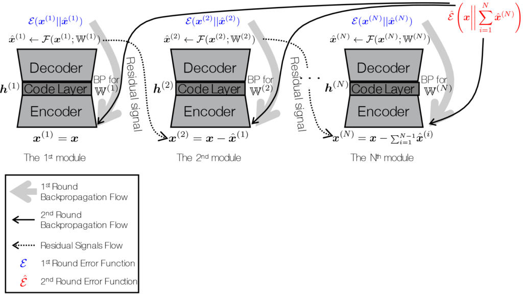
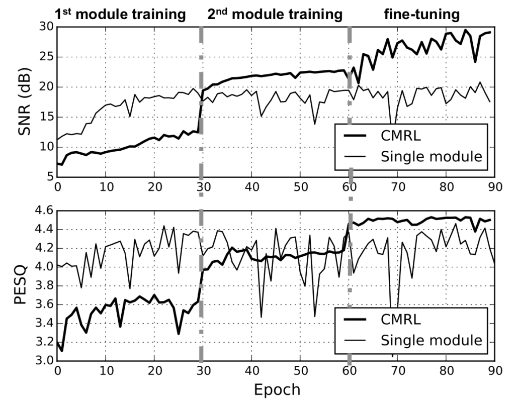
I know it’s a bit more complicated than I explained earlier because it turned out that naïvely learning a new autoencoder for residual coding isn’t the best way—it’s too greedy. For example, if an autoencoder screws up, the next one gets all the burden, while the size of the code grows linearly. So, in addition to the greedy approach, which just works as our fancy initializer, we employ a finetuning step that improves the gross autoencoding quality of all modules by doing backprop over all modules. We call this proposed system Cross-Module Residual Learning (CMRL). Below is the overall architecture of the cascaded autoencoders for residual coding:

What’s even more fun for us is that it turned out that having a linear predictive coding (LPC) block helps the perceptual quality a lot. Since we see LPC as a traditional kind of autoencoding, it’s just another module, like the 0th module, in our cascaded architecture!

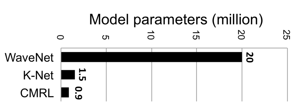
Another thing to note is that we cared much about the model complexity when we designed the system so that the inference during the test time (both encoding and decoding) is not too complicated with small memory footprint. See the comparison on the left with the other codecs:

Please check out our paper² about this project for more details.

---

We found CMRL interesting and versatile. However, it also turned out that its performance in the low-bitrates wasn’t really convincing, while it was able to outperform AMR-WB in the high bitrates. To remedy this, we delved into LPC module further. We originally thought that we may be able to replace LPC with a neural network module, but we wanted to be careful, because it has shown its merit over decades.

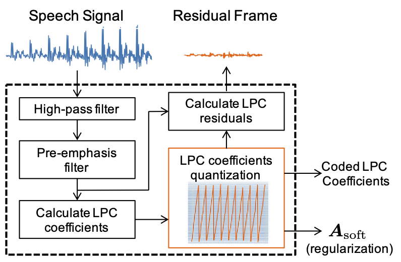
Instead, we made its quantization part trainable. While the LPC residual signals are still covered by our CMRL blocks, the LPC coefficients could have been quantized more carefully than just adopting the AMR-WB’s standard. We wanted to assign bits dynamically to the LPC modules and the CMRL autoencoders, because there must be cases where LPC coefficients matter more than the NN-based autoencoders, vice versa. However, the traditional LPC quantization gives a fixed 2.4 kbps bitrate.

Our Collaborative Quantization (CQ) method approaches to this issue by employing the learnable quantization scheme for the LPC block. Otherwise, the system roughly follows the same argument with CMRL: LPC followed by a bunch of serialized residual coding blocks.

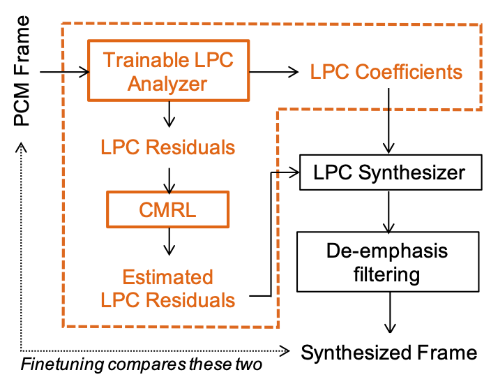
We had to implement LPC so that it runs with Tensorflow (which was kinda painful according to Kai). Anyway, now we can quantize the LPC coefficients along with the other neural networks so that the bit assignment can be done dynamically.

Please check out our paper and code for more details³. The proposed CQ technology successfully improved the performance in the lower bitrate cases.

~9kbps (female) Reference
~9kbps (female) AMR-WB
~9kbps (female) OPUS
~9kbps (female) CMRL
~9kbps (female) CQ
~9kbps (male) Reference
~9kbps (male) AMR-WB
~9kbps (male) OPUS
~9kbps (male) CMRL
~9kbps (male) CQ
~24kbps (female) Reference
~24kbps (female) AMR-WB
~24kbps (female) OPUS
~24kbps (female) CMRL
~24kbps (female) CQ
~24kbps (male) Reference
~24kbps (male) AMR-WB
~24kbps (male) OPUS
~24kbps (male) CMRL
~24kbps (male) CQ

---

1. Srihari Kankanahalli “End-to-end optimized speech coding with deep neural networks.” 2018 IEEE International Conference on Acoustics, Speech and Signal Processing (ICASSP), 2018[↩]
2. Kai Zhen, Jongmo Sung, Mi Suk Lee, Seungkwon Beack, and Minje Kim, “Cascaded Cross-Module Residual Learning towards Lightweight End-to-End Speech Coding,” In Proceedings of the Annual Conference of the International Speech Communication Association (Interspeech), Graz, Austria, September 15-19, 2019 [pdf][↩]
3. Kai Zhen, Mi Suk Lee, Jongmo Sung, Seungkwon Beack, and Minje Kim, “Efficient and Scalable Neural Residual Waveform Coding with Collaborative Quantization,” in Proceedings of the IEEE International Conference on Acoustics, Speech, and Signal Processing (ICASSP), Barcelona, Spain, May 4-8, 2020. [pdf, demo, code][↩]