Neural audio coding is an area where we want to compress an audio signal down to a bitstring, which should be recovered as another audio signal that sounds as similar as possible to human ears, of course, using neural nets. This objective is not that straightforward when it comes to training a neural network that does this autoencoding job, because what I just said in the previous sentence is not well defined as a differentiable loss function.

Neural audio coder, as a machine learning model, can be trained as a parametric function, whose prediction (in the coding case the reconstruction of the input signal) has to be as similar as possible to the target (the input signal before compression). If they are different, the difference is counted as the loss, whose differentiation is propagated back to the network to update the parameters. The tricky issue lies here: Different? Different how?

The loss between the two signals can be computed in various ways: mean-squared error between the time-domain samples, comparison in the frequency domain, taking the log or not, etc. However, none of them is perfect, because human auditory perception is highly subjective and difficult to quantify. For example, even a significantly different pair, in terms of the mean-squared error, can sound indistinguishably similar to a human subject, and vice versa. There have been some efforts in coming up with a more reasonable loss function that aligns better with human auditory perception, but they are somewhat primitive, and not so much work has been done for neural audio coding. Hence, our goal is to come up with a better loss function based on adequate psychoacoustics, which can make the neural audio coders compete with traditional coders.

Meanwhile, in SAIGE we’ve cared so much about the run-time efficiency of deep learning systems. In a typical deep neural network (DNN), there are easily over millions of parameters to work with during a single feedforward pass. What that means is that for a real-time application, there must be millions of floating-point operations at every millisecond or so. We believe that this efficiency issue is severer in neural audio coding, as it ultimately has to deal with real-time decoding for hours on a mobile device. By the way, we’re not talking about efficiency during training. What we care about is the feedforward process during the test time.

There can be a lot of different ways to compress a neural network so that it can enjoy a reduced time, arithmetic, and spatial complexity during the run time. One way would be to use significantly fewer quantization levels to encode the weights, as shown in the bitwise neural networks¹. But, quantization isn’t the only way to compress a net, obviously.

In this project, we took a more fundamental audio-centric approach to the network compression problem, which is eventually related to the loss function. The main idea is to tweak the cost function of a DNN (or actually of any machine learning models) so that the network can focus more on the dimensions that are perceptually meaningful (i.e., audible) while it doesn’t work so hard on the other dimensions that are not. For example, let’s suppose that there is a neural network that produces an -dimensional spectrum . Then, a typical cost function would define the error between the prediction and the ground truth as follows: , with a certain choice of the distance metric . In this formulation, what we could improve is the simple assumption that every frequency subband is equally important. Is this true?

We think the cost function can be better defined. For example, psychoacoustics says that not every frequency subband is equally important². An example would be the simultaneous masking effect, which describes the situation that a peak in the spectrum can mask out the other sound components that are nearby and soft. It’s been the concept widely used in traditional audio coding including MP3. From the perspective of training the neural autoencoders, this is related to an important question: why bother trying to reduce the error that’s inaudible anyway?

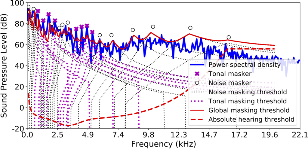
In the figure, the blue curve is the actual energy of the signal over frequencies. The simultaneous masking effect identifies the global masking threshold (red line): the sound component under the curve is inaudible. So, in this figure, the blue line parts that are way under the red line may not need too much attention from the training algorithm, as the network’s mistakes made there can be covered by the threshold (unless the reconstruction error is too much). By calculating the energy ratio between the actual power spectral density of the signal and the global masking threshold, we can come up with a weight vector that works for the given spectrum reconstruction problem: . For example, if is very small, it means that the masking threshold at is substantially higher than the signal, suppressing the contribution of that weights to the total loss. As a result, smaller weights allow the network to make more reconstruction error (but it’s okay if it’s not audible!).

Our conjecture is that the psychoacoustic calibration can improve the sound quality given the same bitrate and network architecture. It is because the adjusted loss function can let the network focus more on the critical components of the input, the more audible parts, which is a smarter way to use bitrate and the other network resources. In other words, the calibrated loss function can reduce the bitrate and network complexity given the same audio quality, as the smaller weights relax the optimization problem.

In addition to the priority weighting scheme explained above, we also propose an additional loss term that simulates MP3’s greedy bit allocation algorithm that minimizes noise-to-mask ratio (NMR), by iteratively demoting the worst reconstruction noise compared against the mask value : . The two proposed loss functions are complementary, as the first one does not explicitly prevent an accidental reconstruction noise peak that can exceed the mask.

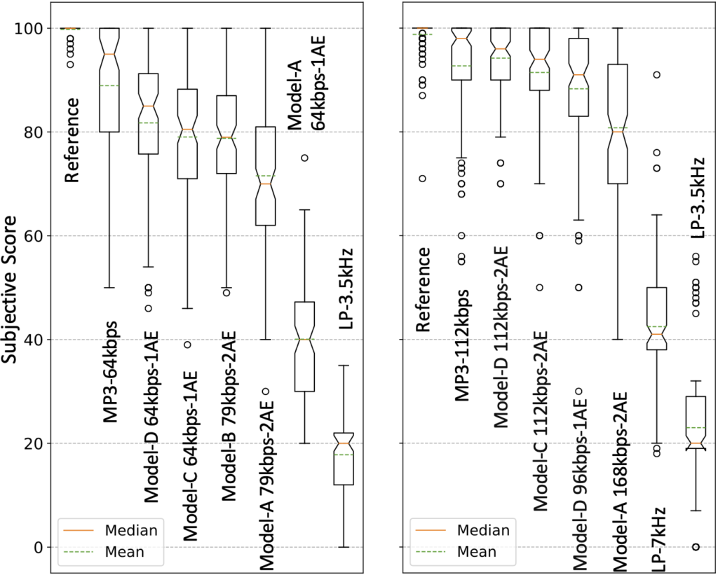
Our subjective tests verify that the proposed method improves the sound quality with reduced model architectures and bitrates.

The Paper

Kai Zhen, Mi Suk Lee, Jongmo Sung, Seungkwon Beack, and Minje Kim, “Psychoacoustic Calibration of Loss Functions for Efficient End-to-End Neural Audio Coding,” IEEE Signal Processing Letters, vol 27, pp. 2159-2163, 2020. [pdf, code]

Source Codes

https://github.com/cocosci/pam-nac

Decoded Samples

The bitrate for uncompressed waveforms is 1.411 Mbps, the same as CD’s with the stereo setup. For the mono setup in this work, the uncompressed bitrate is 705.6 kbps.

Low Bitrates, 32 kHz

• Model-A (NAC with MSE loss), 64 kbps; 0.45M parameters
• Model-A (NAC with MSE loss), 79 kbps; 0.9M parameters
• Model-B (Model-A loss + mel-scale), 79 kbps, 0.9M parameters
• Model-C (Model-B loss + priority weighting), 64 kbps, 0.45M parameters
• Model-D (Model-C loss + noise modulation), 64 kbps, 0.45M parameters
• MP3, 64 kbps

Low bitrates example #1

Low bitrates example #2

Low bitrates example #3

High Bitrates, 44.1 kHz

• Model-A (NAC with MSE loss), 168 kbps; 0.9M parameters
• Model-C (Model-A loss + mel-scale and priority weighting), 96 kbps, 0.45M parameters
• Model-C (Model-A loss +mel-scale and priority weighting), 112 kbps, 0.9M parameters
• Model-D (Model-C loss + noise modulation), 96 kbps, 0.45M parameters
• Model-D (Model-C loss + noise modulation), 112 kbps, 0.9M parameters
• MP3, 112 kbps

High bitrates example #1

High bitrates example #2

High bitrates example #3

1. Minje Kim and Paris Smaragdis, “Bitwise Neural Networks,” International Conference on Machine Learning (ICML) Workshop on Resource-Efficient Machine Learning, Lille, France, Jul. 6-11, 2015. [pdf][↩]
2. Painter and A. Spanias, “Perceptual coding of digital audio,” Proceedings of the IEEE, vol. 88, no. 4, pp. 451–515, 2000.[↩]