Motivation

We bring the cool generative power of a diffusion model to speech coding. We call our codec LaDiffCodec as it is actively using the concept of latent diffusion¹ in order to incorporate a generative model to the neural speech codec, especially as a module to perform de-quantization, which is a bottleneck of the performance.

When generative models were first introduced to speech coding, it was used as the main decoding module. But, instead of recovering the waveform from the quantized code as in supervised models², generative models, such as WaveNet, were employed to “synthesize” an utterance³. In order to prevent the autoregressive model from generating a new utterance that’s different from the original input, though, the synthesis process was “conditioned” by the code extracted from the input.

Although this kind of codec works pretty well, exceeding the traditional speech codec’s performance by a great margin, the idea of generating samples one-by-one is a little time and resource-consuming operation. Instead, it might be better to generate something in the latent space, in a frame-by-frame manner. That’s where the idea of predicting in the coded space came from as in^{4 5}.

Meanwhile, LaDiffCodec is also designed to address the common issues in the waveform codecs: quantization messes up the codec’s performance. For example, it is easy to empirically show that an autoencoder can do a great job in reconstructing the input signal as it is, if no quantization of the bottleneck features is involved in. Conversely, since modern neural speech codecs are with an ultra-low bitrate (as low as 1 kbps), recovering continuous signals from such a heavily quantized code is a very challenging task.

The Proposed LaDiffCodec

LaDiffCodec consists of three modules.

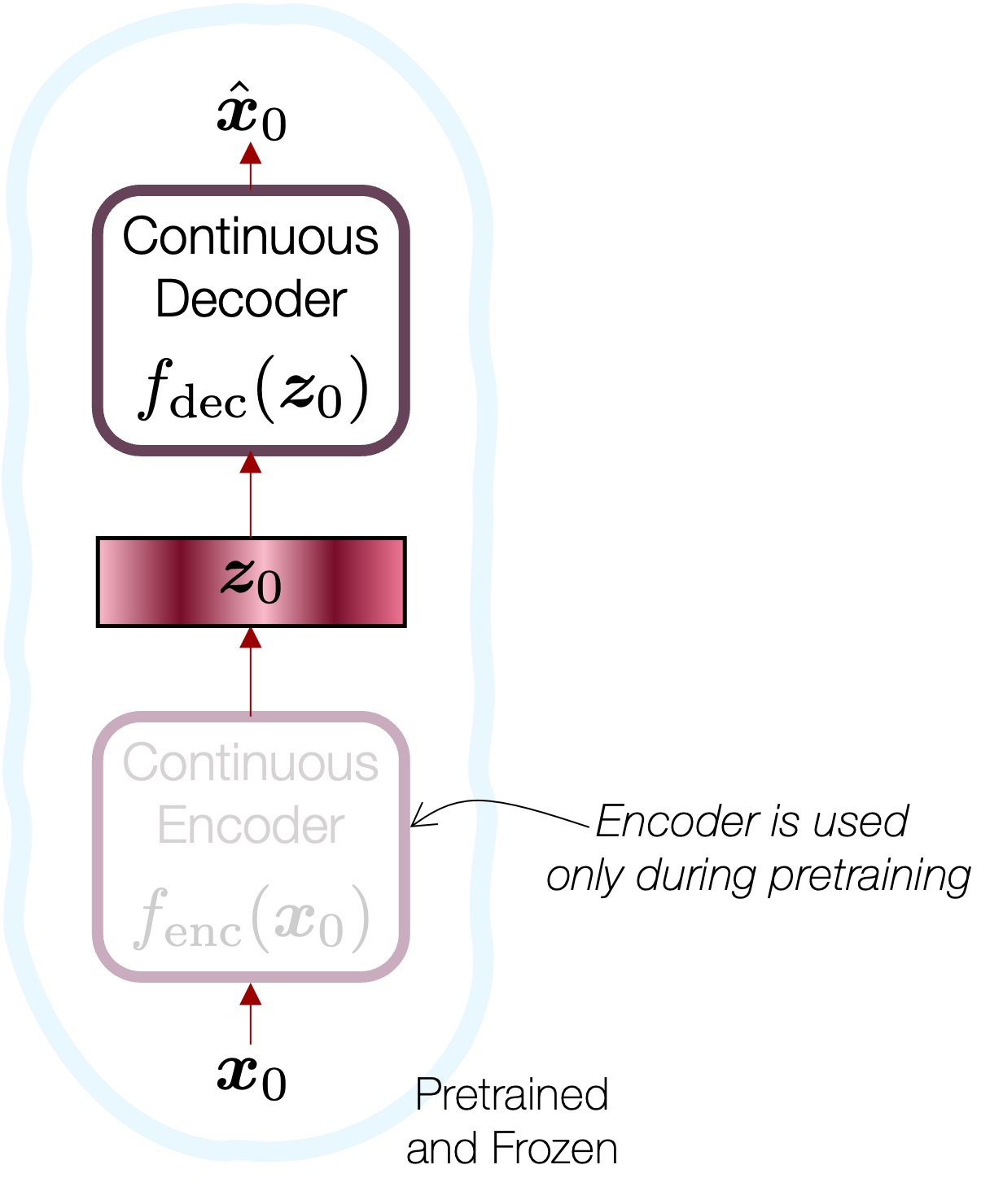
First, we train a continuous autoencoder without any quantization. Its reconstruction must sound great (i.e., transparent), but, you know, it’s useless as a codec as the bottleneck feature is not quantized. It might be with a too high bitrate due to the floating-point code vectors. We employ an EnCodec(())-like architecture for this, but without doing any quantization.

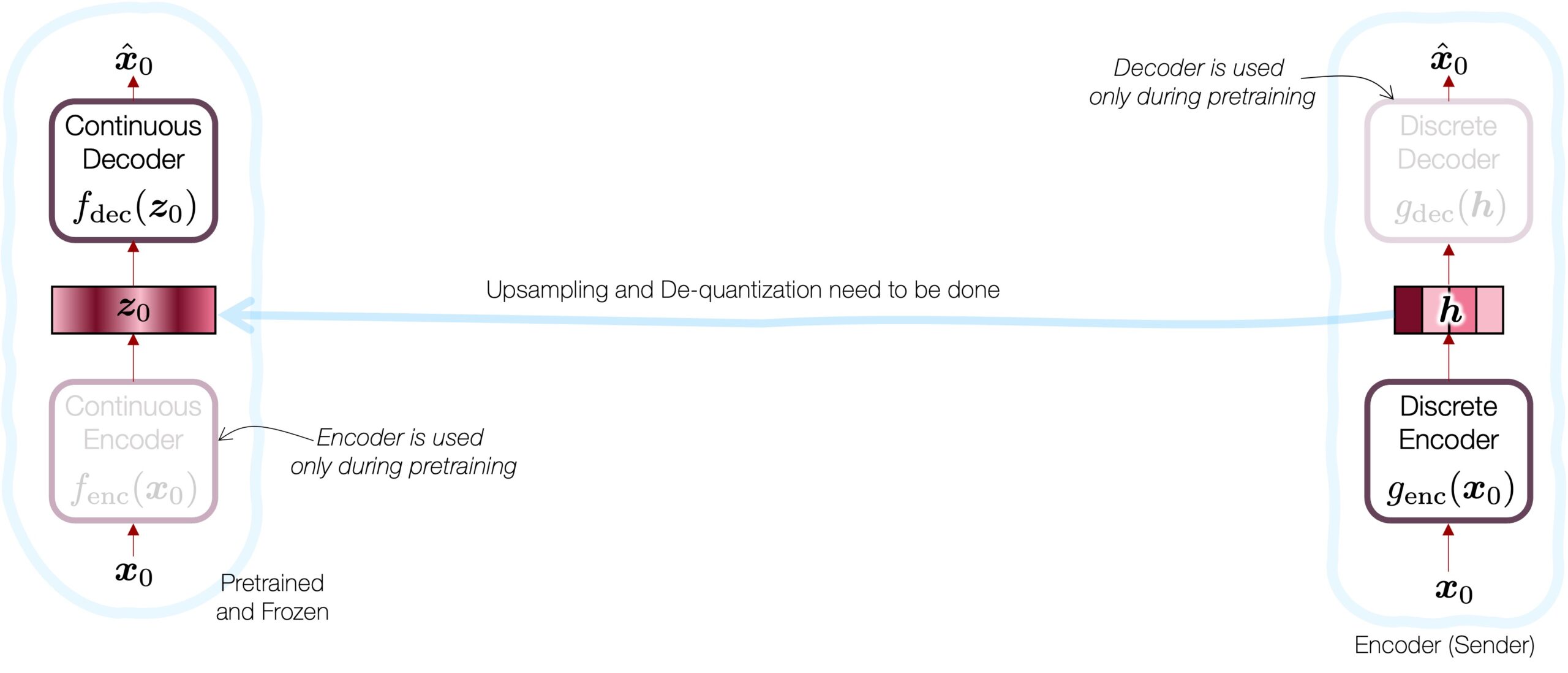
Second, we train a regular (i.e., discrete) codec with proper quantization (i.e., residual vector quantization) in the middle. This might be very similar to the EnCodec baseline. It is decent, but compared to the autoencoder output, it’s far from perfection.

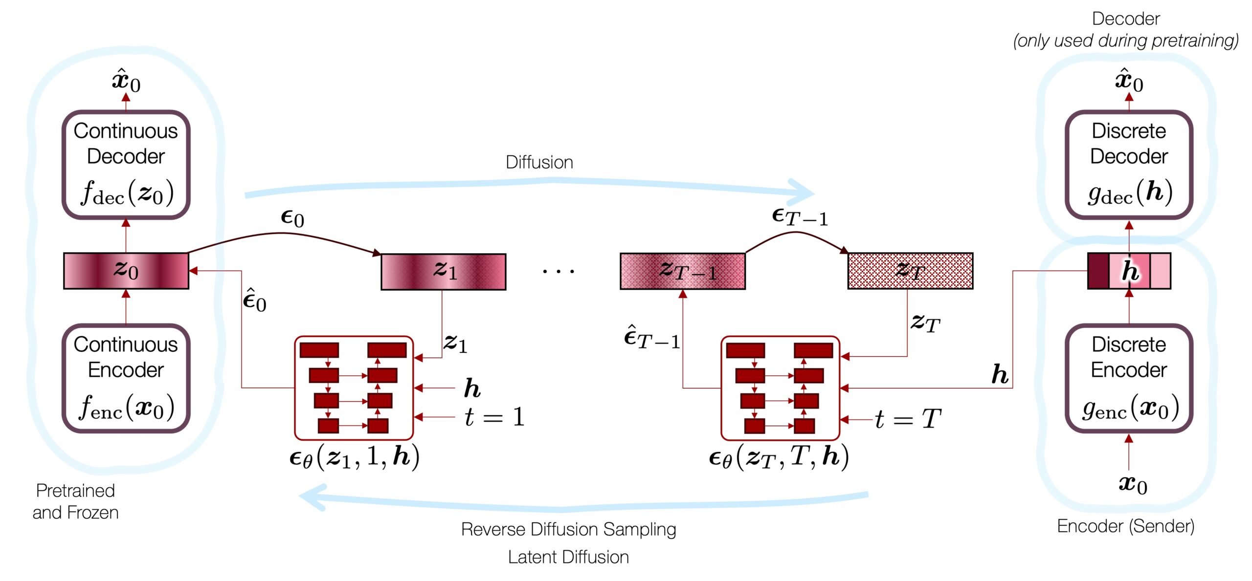
Third, we train a latent diffusion model that works in the latent space. This latent model is basically the glue that puts the two EnCodec variations together, while overcoming their drawbacks. Basically, the latent diffusion model is trained to “generate” the continuous latent vector , which is the input to the continuous decoder . We know that the result will sound great if is a proper representation of the input signal , because no quantization is involved in. However, the diffusion model in the middle knows nothing about what should sound like, so it will just synthesize a “plausible” one which doesn’t sound like the original speech. Hence, we need to condition this diffusion model by using the quantized code produced by the discrete codec’s output . Since all this generation process is happening in the latent space, we call it latent diffusion codec, or LaDiffCodec.

In other words, to summarize, we want to stitch the discrete encoder continuous decoder and , because the former is good at compressing the signal, while the latter guarantees quality reconstruction. However, it’s impossible because the discrete code and continuous code don’t reside in the same space. The latent diffusion model comes in to play the moderator’s role, and converts the quantized code into the continuous version. What’s nice about all this diffusion process is that it’s still a generative model, leaving a lot of liberty to the de-quantization process to be creative and overcome the loss and artifact lying in the discrete coding process.

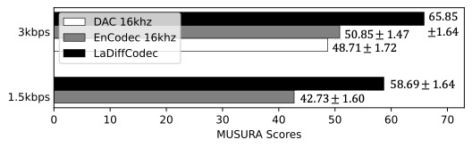
Please check out the subjective listening test results (MUSHRA-like), where we can see that the proposed LaDiffCodec outperforms a couple of recent neural speech codecs.

For more details about LaDiffCodec, including the midway infilling algorithm that dramatically reduces the number of reverse diffusion steps, please take a look at our paper.

Paper

• Haici Yang, Inseon Jang, and Minje Kim, “Generative De-Quantization for Neural Speech Codec via Latent Diffusion,” in Proceedings of the IEEE International Conference on Acoustics, Speech, and Signal Processing (ICASSP), Seoul, Korea, Apr. 14-19, 2024 [pdf, demo, code].

Sound Examples

Example #1

Example #2

Ablation of the Midway Infilling Algorithm

The following sequence of samples are synthesized using the proposed midway-infilling algorithm with different interpolation rates . The larger is, the more the condition branch (i.e., the quantized code) participates in the sampling procedure, which improves the “correctness” of the synthesized examples at the cost of reduced “naturalness.” All of them took 100 steps for sampling. We also provide the samples using DDPM sampling (baseline) with 1000 steps for comparison.

Example #1 at 1.0 kbps

“Sufficient to serve with five or six mackerel.”
(In the baseline result and some other infilling results, the word “serve” is mispronounced.)

Source Codes

https://github.com/haiciyang/LaDiffCodec

1. R. Rombach, A. Blattmann, D. Lorenz, P. Esser, and B. Ommer, “High-resolution image synthesis with latent diffusion models,” in Proceedings of the IEEE/CVF conference on computer vision and pattern recognition, 2022, pp. 10684–10695.[↩]
2. S. Kankanahalli, “End-to-end optimized speech coding with deep neural networks,” in Proceedings of the IEEE International Conference on Acoustics, Speech and Signal Processing (ICASSP), 2018.[↩]
3. W. B. Kleijn, F. S. C. Lim, A. Luebs, J. Skoglund, F. Stimberg, Q. Wang, and T. C. Walters, “WaveNet based low rate speech coding,” in Proceedings of the IEEE International Conference on Acoustics, Speech, and Signal Processing (ICASSP), 2018, pp. 676–680.[↩]
4. H. Yang, K. Zhen, S. Beack, and M. Kim, “Source-aware neural speech coding for noisy speech compression,” in Proc. of the IEEE International Conference on Acoustics, Speech, and
   Signal Processing (ICASSP), 2021.[↩]
5. Xue Jiang, Xiulian Peng, Huaying Xue, Yuan Zhang, and Yan Lu, “Latent-Domain Predictive Neural Speech Coding,” IEEE/ACM Transactions on Audio, Speech and Language Processing. 31 (2023), 2111–2123.[↩]