We have cared much about the efficiency of the machine learning inference process. As a part of this effort, we recently came up with a hash code-based source separation system, where we used a specially designed hash function to increase the source separation performance and efficiency.
KNN Source Separation
Our idea starts from the nearest neighbor search. Imagine you have a set of mixture spectra, whose target clean sources are already known. From them, we can construct a rather exhaustive dictionary of mixture spectra in the frequency domain (the row vectors of the pink matrix in the figure below).
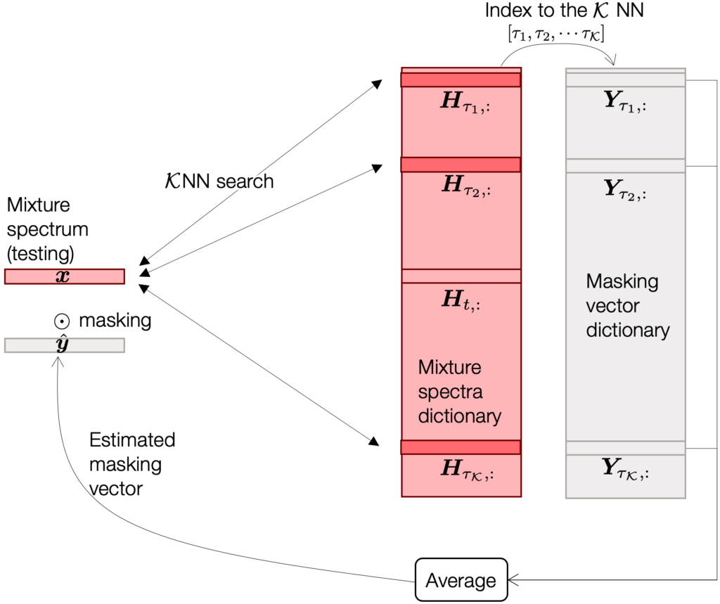
For a given test spectrum  , this naïve separation system first finds out a few most similar spectra (e.g., by doing inner product between and all the row vectors of
  . Since is a large dictionary, hopefully there are a few items that are similar enough. If the search is successful, then the rest of the job is a done deal, because we already know the corresponding source spectra of all the dictionary items. We can simply collect the source vectors corresponding to the KNN dictionary items, and then average them out1.
Although this naïve idea works quite well (we could get about 9.66 dB improvement in terms of signal-to-noise ratio), we found it disturbing, because the KNN search for every incoming test spectrum is unrealistically expensive.
A hashing-based speed-up!
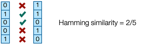
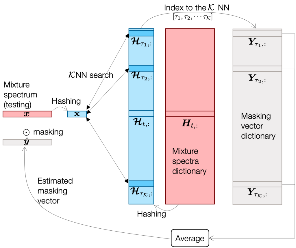
That’s why we need a hashing technique. As a function, hashing can convert an input multi-dimensional vector into a bitstring  :
:  . So what? When we compare two bitstrings we can do it by using simple Hamming distance calculation, which is a bitwise operation (see the figure below for an example).
For example, if we use locality sensitive hashing (LSH)2 3, the hash function randomly generates a projection matrix  and multiply it to the input vector to take the sign of the projected coefficients:
  . Hence, if there are
  rows in , we get bipolar binary values4. For example, if we start from a 513-dimensional Fourier magnitude coefficients
  and then use
  we can reach 8.75 dB improvement. It’s quite a good amount of reduction from 513 floating-point values down to 150 binary values in terms of both spatial and computational complexity.
All this hashing-related argument is cool, but we wanted to do it better. Obviously, while simple and effective, LSH might not be the best hash function for my problem, since it’s purely based on a bunch of random projections. What if there is another hash function that works as good as this  LSH case, but with much smaller , such as only 25 bits?
Limitations of LSH
Let’s revisit the LSH algorithm to understand its limitations. Again, LSH is based on random projections. It means that for a pair of very close examples, it’s hard for them to be on the opposite sides (positive and negative) after the projection, as illustrated in the following figure.
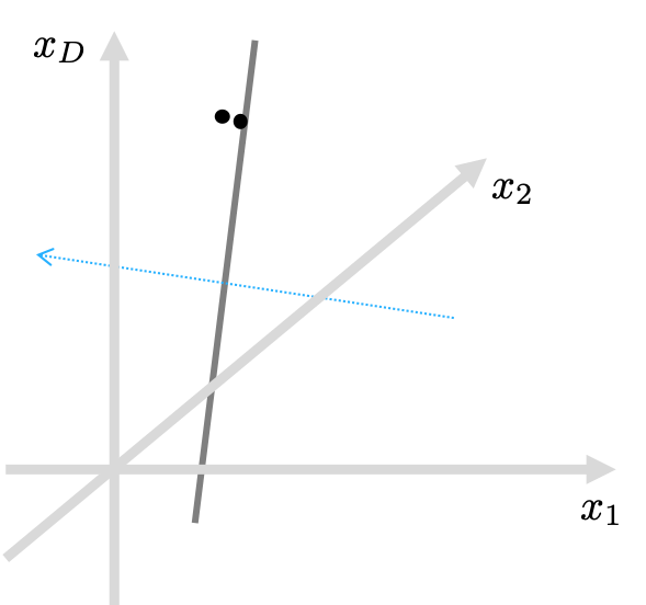
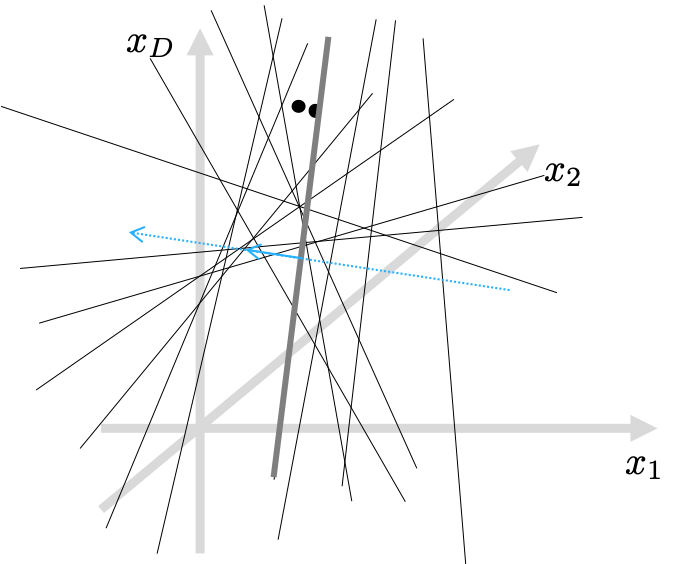
I’d like to call these random projections “a drunk knight’s swinging experiment.” Imagine a pair of apples hanging in the air, but their distance is only an inch. It might be difficult for the drunk knight to swing a sword in-between the apples, ’cause HE IS DRUNK! That’s why LSH produces similar bitstrings for originally similar input vectors.
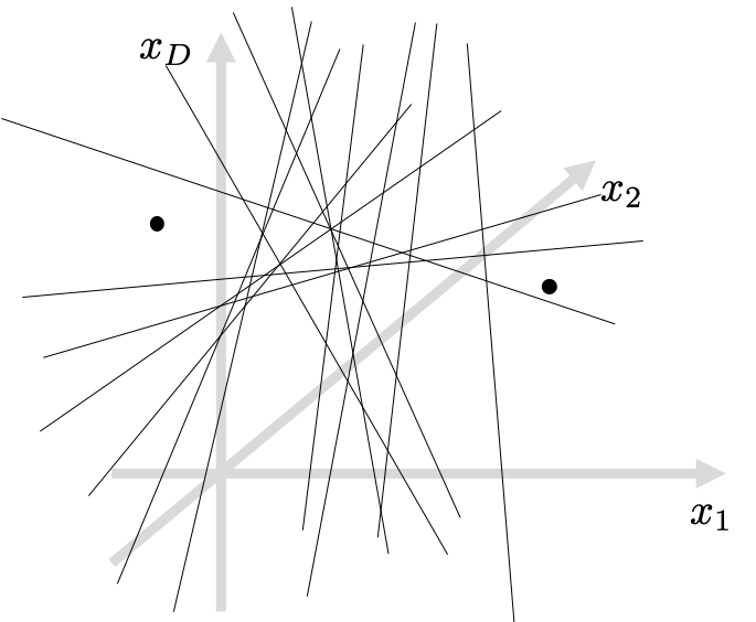
On the other hand, LSH CAN create discriminative bitstrings, when the apples are far away. In other words, LSH projections are more probable to generate differently signed bits if the compared examples are far from each other in the original data space. See the example below.
Boosted LSH
To this end, we developed a new LSH algorithm, called Boosted LSH (BLSH), where we introduce the AdaBoost algorithm to train the projections. With boosting, what we can do is to learn the projection vectors “one-by-one” in the order of their importance. Let’s start by learning the first projection vector. Even though it’s going to give us just a sign for each of the examples, it should best represent the similarity and dissimilarity of all the spectra. The learning is relatively simple, because we will eventually learn a projection vector followed by a nonlinearity function, i.e., the sign function. Ring a bell? It’s just a perceptron! For the next one, according to the boosting scheme, we will focus on the examples that are mis-represented by the first code, by focusing more on them. By doing so, whenever we add a new perceptron, or a weak learner, it’s to make up the mistakes the previously learned weak learners have made so far.

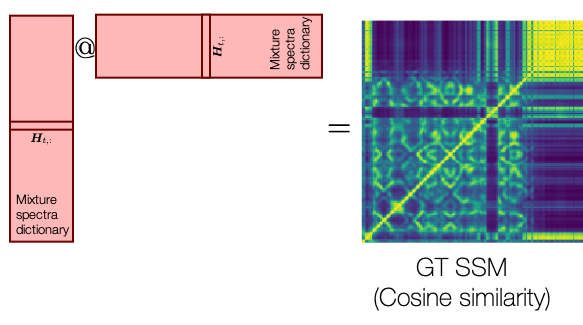
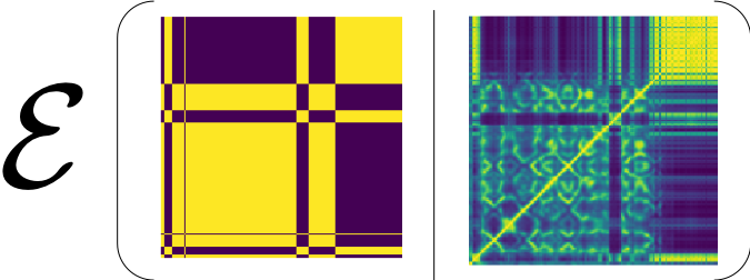
Our challenge is that we don’t do classification, but the KNN source separation. So, we cannot check on the “misclassification” error to pay different attentions to the examples. Instead, we will use the pairwise similarity between the original spectra as our target: for a given pair of spectra in the matrix, if the pairwise Hamming similarity of the so-far learned hash codes is off from the original, we give a large weight to that pair to instruct the next perceptron to pay attention to it. Here’s the target of our training, the self-similarity matrix (SSM):
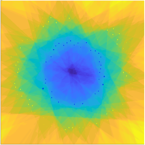
Given this ground-truth SSM, our first perceptron should give us a binary value per example, which as a feature should try to catch up the shape of the GT SSM. The first hash code we learn from the first perceptron indeed recovers some large structures in the GT SSM:
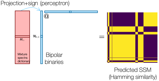
When we train this first perceptron, we repeatedly perform a prediction using current perceptron weights (or the projection vector), and then the predicted bipolar binary values construct the predicted SSM. The predicted SSM is compared against the ground-truth SSM to compute the loss, which is backpropagated to updated the perceptron.
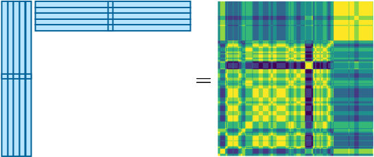
For the following perceptrons, whenever we add more of them to the pool of weak learners, they gradually improve the performance, meaning the recovered SSM looks more similar to the original. For the 5th perceptron, for example, it looks like this:
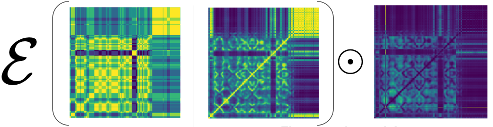
Learning this  -th perceptron is a little different from the very first perceptron training, as we need to give different weights to the “misclassified” examples. In our case, out of the comparison of SSMs, we can identify some SSM elements that are not doing well. It’s of course different from “misclassification” concept, but equally effective for our boosting algorithm. After all, when we compute the loss, we element-wise multiply this weight matrix as follows:
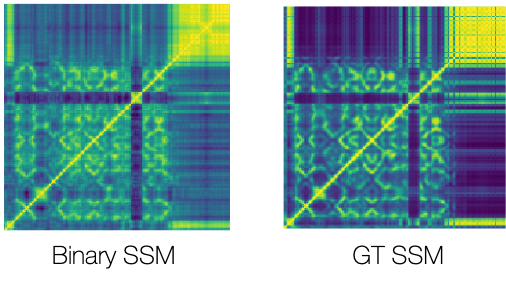
Finally, below is the binary SSM we compute after learning 100 projections along with the ground truth side-by-side:
Experimental results
Let’s take a look at this graph that summarizes the behavior of our hashing-based source separation model.
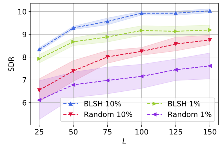
First off, all the models enjoy the improved separation performance (in terms of signal-to-distortion ratio) by using longer hash codes ( denotes the number of bits). But, the proposed BLSH methods (blue and green) consistently outperform the ordinary random projection-based LSH (red and purple). What’s more is about the size of the matrix. If we use only 1% of available mixture spectra for our dictionary, the random projection-based LSH suffers a lot from the low performance and an increased uncertainty (purple). It means that, depending on how the random projection matrix is sampled, the performance varies significantly (see the large confidence intervals). On the other hand, with our BLSH algorithm, although its separation quality is degraded when we use too few examples (1%), the confidence interval is much narrower (green), showcasing that BLSH is free from the performance fluctuation issue that LSH suffers from.
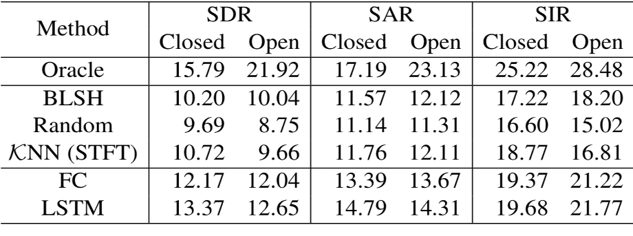
In the table below, we compare BLSH with various other setups, including an open case (where the test signals’ noise sources are not known to the hashing algorithm). Surprisingly, BLSH outperforms an STFT-based baseline. It means that BLSH succeeded to learn better features than the raw Fourier coefficients. It’s still far from deep learning models’ performance, but considering the efficiency, BLSH is promising for source separation in resource-constrained environments.
 .
.Audio examples
In the following examples, we will see the merit of BLSH over LSH, because for BLSH the bit length  , while LSH had to use 125 bits to do the similar-quality separation. The point is that BLSH is still effective in lower-bit representations.
 . The SDR of the reconstruction is 8.95 dB. The reconstruction SDR is 8.33dB.
Below we introduce a few other examples as the BLSH-based separation results. On the left, they are the mixture input to the system, and the corresponding separation results are on the right.
Papers
For more details please take a look at our ICASSP 2020 paper, which was nominated for the Best Student Paper Award5.
For a more in-depth analysis, and interpretation from the manifold learning-perspective and kernel methods, are available in our journal paper: 6
Source Codes
We also open-sourced the project.
- The ICASSP version: https://github.com/sunwookimiub/BLSH
- The journal version: https://github.com/kimsunwiub/BLSH-TASLP
Virtual presentation at ICASSP 2020
This material is based upon work supported by the National Science Foundation under Grant Number 1909509. Any opinions, findings, and conclusions or recommendations expressed in this material are those of the authors and do not necessarily reflect the views of the National Science Foundation.
- In this system, we used ideal binary masks (IBM) of the corresponding mixture instead of the direct source estimates.[↩]
- P. Indyk and R. Motwani, “Approximate nearest neighbor – towards removing the curse of dimensionality,” in Proceed- ings of the Annual ACM Symposium on Theory of Computing (STOC), 1998, pp. 604–613.[↩]
- M. Datar, N. Immorlica, P. Indyk, and V. S. Mirrokni, “Locality-sensitive hashing scheme based on p-stable distribu- tions,” in Proceedings of the twentieth annual symposium on Computational geometry. ACM, 2004, pp. 253–262.[↩]
- +1’s and -1’s.[↩]
- Sunwoo Kim, Haici Yang, and Minje Kim, “Boosted Locality Sensitive Hashing: Discriminative Binary Codes for Source Separation,” in Proceedings of the IEEE International Conference on Acoustics, Speech, and Signal Processing (ICASSP), Barcelona, Spain, May 4-8, 2020. [pdf, code][↩]
- Sunwoo Kim and Minje Kim, “Boosted Locality Sensitive Hashing: Discriminative, Efficient, and Scalable Binary Codes for Source Separation,” IEEE/ACM Transactions on Audio, Speech, and Language Processing, vol. 30, pp. 2659-2672, Aug. 2022 [pdf, code][↩]